

Families planning to retire early often face a liquidity problem when most of their savings are in tax-advantaged retirement accounts. They may have substantial net worth but not enough accessible cash to cover living expenses before age 59½.
Consider David and his family, who plan to retire at the end of 2026:
Age: 52/53
Net Worth: $2.3M
Assets: $300K in a taxable brokerage account and $2M in a tax-deferred 401(k)
Annual Living Expenses: $75K (in today’s dollars)
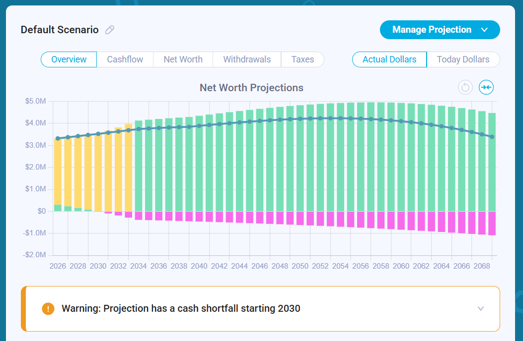
David starts by modeling a retirement scenario in which the family covers living expenses using only their taxable brokerage account. The problem is that the $300K runs out within the first 4 years, leaving the family with a growing cash shortfall between 2030 and 2034, even though they still have substantial savings in their 401(k).
The projection chart below illustrates the problem. Green bars show liquid assets, yellow bars represent non-liquid net worth, and bright pink bars indicate cash shortfalls:
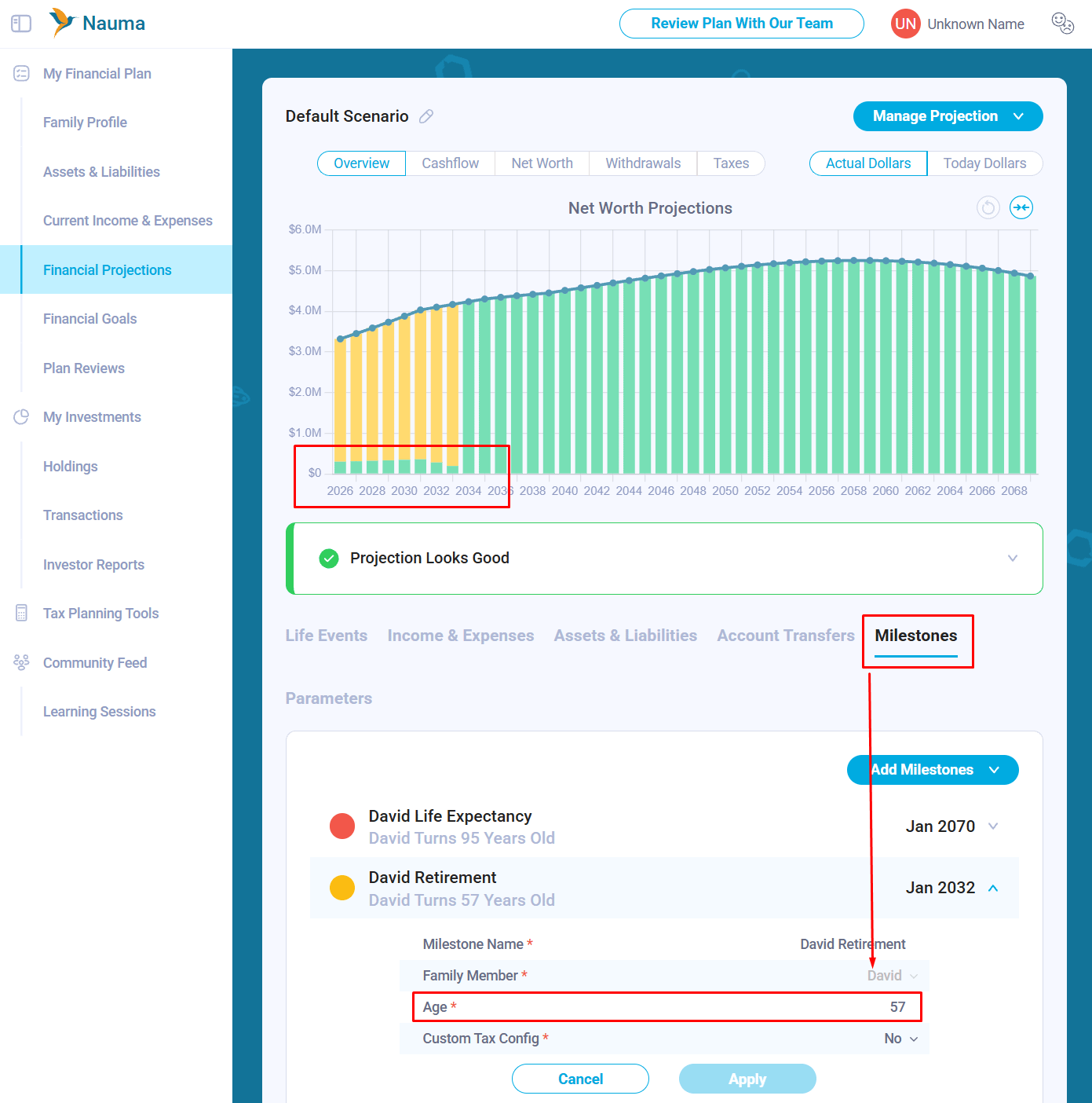
Testing a 5-year delay in retirement (working until age 57) eliminates the liquidity shortfall, but it introduces high opportunity cost. Under that scenario, David gives up 5 prime years of early retirement only to end his financial plan with roughly $1.6M (assuming conservative 4% annual growth rate in retirement) in unspent, inflation-adjusted assets.
Rather than delaying retirement unnecessarily, David turns to Section 72(t) of the IRS tax code, specifically Substantially Equal Periodic Payments (SEPP), to model how he can unlock his 401(k) penalty-free.
IRS Methods for Accessing Tax-Deferred Accounts
SEPP allows early retirees to take penalty-free distributions from retirement accounts before 59½, if withdrawals follow a strict schedule for at least 5 years or until reaching age 59½ (whichever is longer). The IRS permits three distinct calculation methods:
RMD (Required Minimum Distribution) Method: Calculates variable annual withdrawals by dividing the prior year’s account balance by an IRS life expectancy factor. Because the amount recalculates every year, payments fluctuate with market performance.
Fixed Amortization Method: Generates a fixed annual payment by amortizing the account balance over a chosen life expectancy using an IRS-approved interest rate (such as the federal midterm rate).
Fixed Annuitization Method: Produces a fixed annual payment similar to amortization, but derives the distribution using an annuity factor from an IRS mortality table.
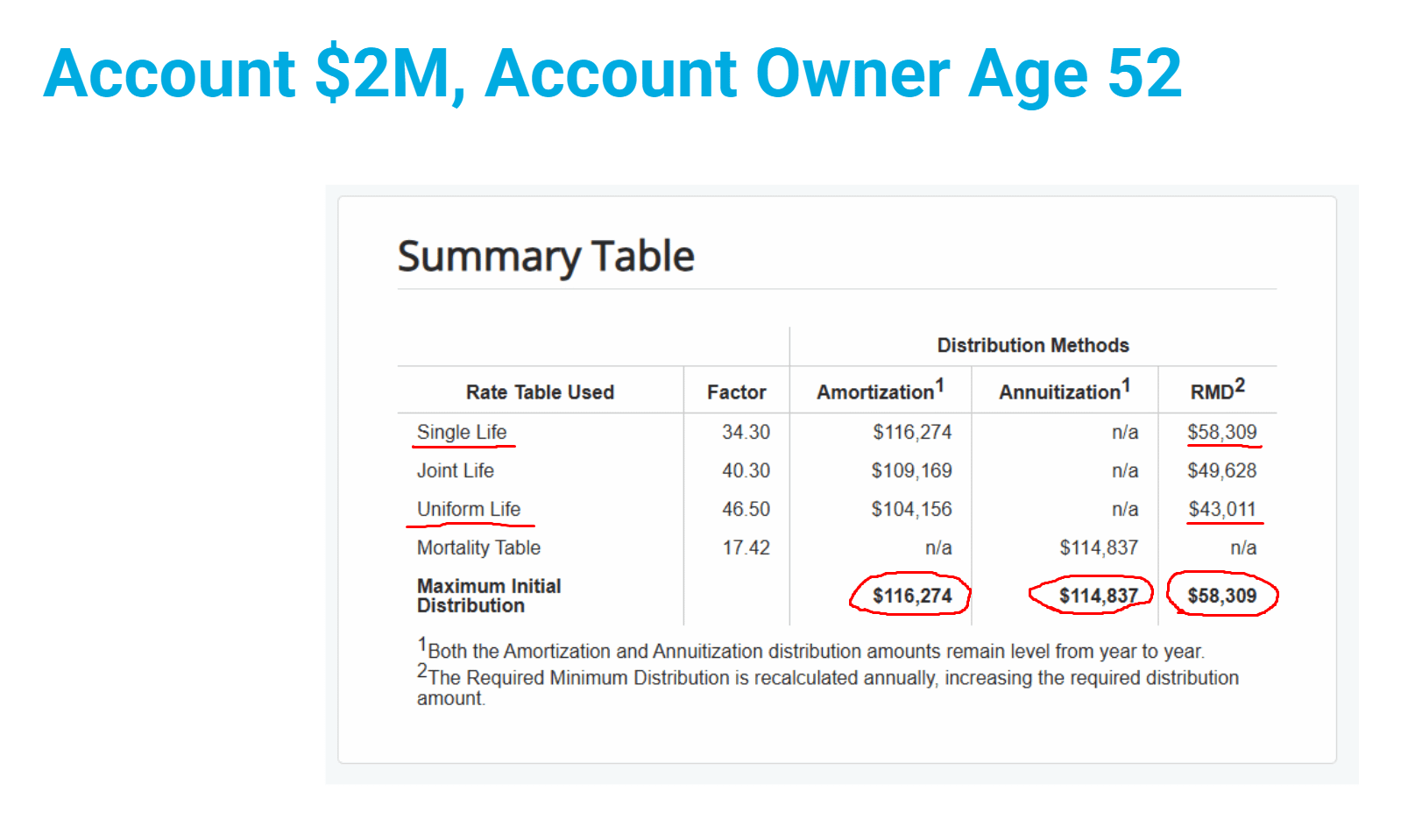
Distribution amounts are also governed by which IRS life expectancy table is applied. The Single Life table generally produces the highest annual payouts, whereas the Joint Life and Uniform Life tables generate lower, more conservative withdrawals. DIY planners can also control payout sizes by splitting a large 401(k) or IRA into separate accounts and applying SEPP to only a portion of their total balance.
Trade-Offs: Market Risk vs. Income Control
As David tests different SEPP parameters in his plan, each method introduces a distinct trade-off between Sequence of Return Risk and cash-flow predictability:
Mitigating Market Risk: The RMD method is best suited for retirees concerned about a market downturn early in retirement. Because distributions recalculate annually, a drop in portfolio value reduces the required withdrawal the following year, protecting the underlying principal from accelerated depletion.
Maximizing Control: The Fixed Amortization and Fixed Annuitization methods allow retirees to lock in higher, predictable annual income by utilizing current IRS interest rates. However, because the withdrawal amount stays fixed regardless of market performance, a severe downturn exposes the portfolio to heightened sequence of return risk.
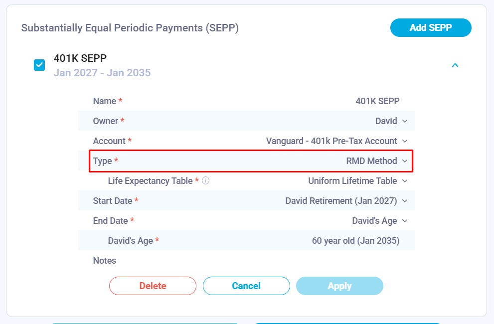
Applying these methods to David’s $2M 401(k) at age 52, using the Uniform Life table and running payments until age 60, produces two very different financial trajectories:
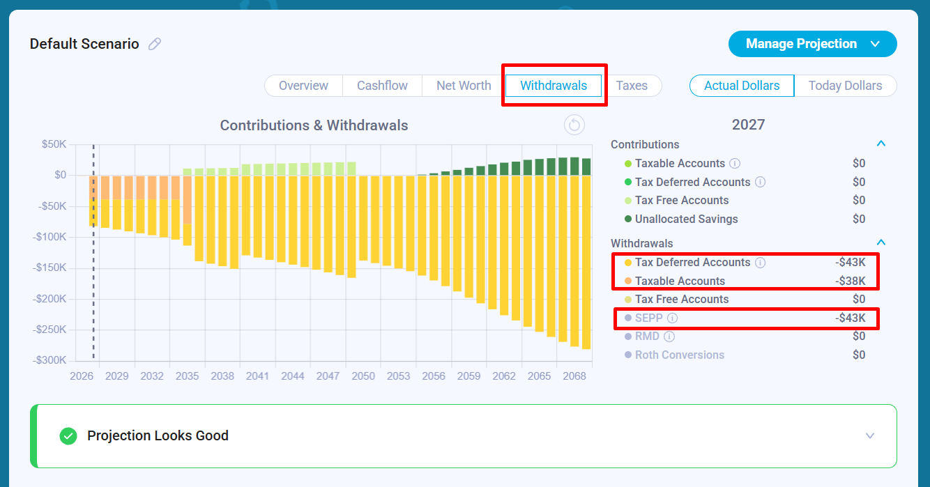
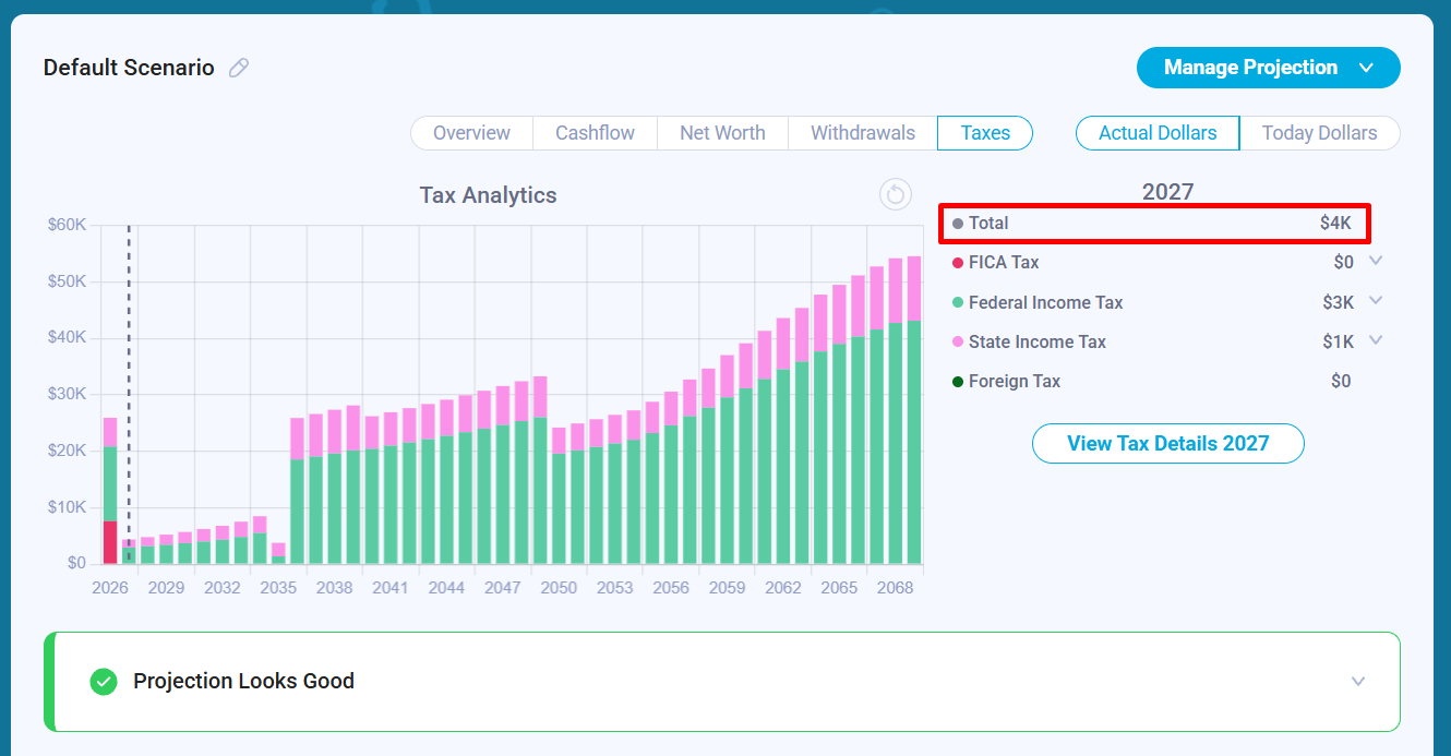
Scenario A: The RMD Method: Generates roughly $43K in annual SEPP distributions. Because the family needs approximately $86K per year to cover their $75K in living expenses plus taxes, David’s model pulls the remaining balance from their taxable brokerage account. Blending taxable and tax-deferred withdrawals keeps annual taxes low (around $4K in the later bridge years) until SEPP ends at age 60. Once they exhaust their taxable account in their early 60s and shift fully to tax-deferred withdrawals, their annual tax bill jumps to roughly $26K.
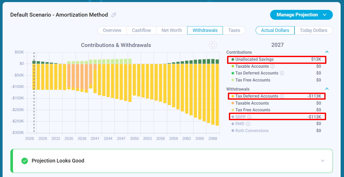
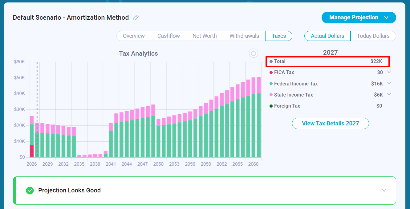
Scenario B: The Fixed Amortization Method (5% interest rate): Generates $113K in annual SEPP distributions. This single distribution covers all living expenses and taxes on its own, leaving roughly $13K in annual surplus that gets reinvested into their taxable brokerage account. However, recognizing higher ordinary income early pushes their annual taxes up to roughly $22K during the SEPP years. Once SEPP ends at age 60, the family switches to spending down their grown taxable account, dropping their annual tax liability to roughly $1K until those funds are depleted.
Selecting the right SEPP calculation method directly impacts a household’s lifetime tax liability and terminal net worth. Across long-term models, the spread between distribution strategies can reach $200K to $400K in nominal dollars by the end of a financial plan. This gap is primarily driven by over-distributing: setting unnecessarily high fixed payments increases ordinary income and forces the family to use higher marginal tax brackets. Conversely, setting SEPP payouts closer to actual cash-flow needs preserves tax-deferred compounding and allows retirees to use lower marginal tax rates over time.
Secondary Impacts: Tax Sequencing and Roth Conversions
Adding SEPP distributions changes a household’s taxable income profile, meaning any existing Roth conversion schedule has to be recalculated from scratch.
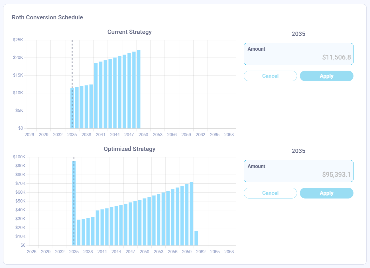
In David’s original baseline model without SEPP, low taxable income in early retirement pointed toward converting small amounts (roughly $11K) each year. Once he layers in SEPP distributions and re-runs his Roth conversion optimizer up to the 24% federal tax bracket, the Roth strategy changes because SEPP fills up his lower tax brackets between ages 52 and 59½.
Ultimately, there is no single “best” SEPP strategy, only trade-offs between early cash flow, market risk, and lifetime tax drag. Modeling these variables side-by-side ensures you don’t accidentally trade a short-term liquidity crunch for a six-figure tax bill down the road.
About The Author
Alex Sukhanov, founder of Nauma, a financial planning platform built for people in tech and high-net-worth families. Alex previously worked at Google and started Nauma to help more people in tech make better financial decisions and achieve more in their lives. You can reach out to Alex on linkedin.
Nauma is supported entirely by its users: no commissions, no affiliate incentives, and no financial products to sell. Built as an independent software platform rather than a traditional advisory firm, Nauma is designed to give tech professionals the tools and modeling clarity to evaluate their own equity, tax, and retirement scenarios.

Important Disclosures: This article is provided for educational and informational purposes only and does not constitute investment, tax, or legal advice. The case study and financial projections presented are hypothetical simulations based on specific user-defined assumptions (including a 4% annual portfolio return, a 5% Section 72(t) interest rate, 3% inflation and current federal tax brackets). Nauma is a financial technology software company, not a registered investment adviser, broker-dealer, or tax firm.